What is Google Analytics?
Google Analytics is a web analytics service offered by Google that tracks and reports website traffic. It is currently a platform in the Google Marketing Platform brand. Google Analytics is the most widely used web analytics service on the web. It is a powerful tool that provides insights into how users interact with your website, allowing you to make data-driven decisions to improve user experience and optimize your marketing efforts. Google Analytics 4 (GA4) is the latest version of Google Analytics, which focuses on event-based tracking and provides more advanced features for analyzing user behavior across different platforms.
The googleAnalyticsR package
The googleAnalyticsR package is an R client for the Google Analytics API. It allows you to access and analyze your Google Analytics data directly from R, making it easier to integrate web analytics into your data analysis workflow. The package provides functions to authenticate with your Google account, retrieve data from Google Analytics, and perform various analyses on the data.
Getting started with googleAnalyticsR
ga_auth(email = "seandavi@gmail.com")#> ℹ Authenticating using ga4-api-accessor@bioconductor-ga4-home.iam.gserviceaccount.com
account_list <- ga_account_list("ga4")

## account_list will have a column called "propertyId"
account_list$propertyId
#> [1] "388188354"

## View account_list and pick the one that you want to use
## In this case, we will use Bioconductor
ga_id <- 388188354
The resulting res object will contain the data for the specified date range, metrics, and dimensions. You can view the first few rows of the data using the head() function.
library(lubridate)
#>
#> Attaching package: 'lubridate'
#> The following objects are masked from 'package:base':
#>
#>     date, intersect, setdiff, union

start_date <- Sys.Date() - 365
end_date <- Sys.Date() - 1


daily_user_country_data <- ga_data(
    propertyId = ga_id,
    dimensions = c("date", "newVsReturning", "country"), # Added dimensions
    metrics = c("activeUsers", "sessions"), # Example metrics
    date_range = c(start_date, end_date),
    limit = -1
)
#> ℹ 2025-12-05 20:41:30.463384 > Downloaded [ 82263 ] of total [ 82263 ] rows
library(ggplot2)
library(zoo)
#>
#> Attaching package: 'zoo'
#> The following objects are masked from 'package:base':
#>
#> as.Date, as.Date.numeric
library(dplyr)
#>
#> Attaching package: 'dplyr'
#> The following objects are masked from 'package:stats':
#>
#> filter, lag
#> The following objects are masked from 'package:base':
#>
#> intersect, setdiff, setequal, union
# Group by user type and country, then calculate rolling average
moving_avg_data <- daily_user_country_data |>
arrange(date) |>
group_by(newVsReturning, country) |>
mutate(
activeUsers_7day_avg = rollmean(activeUsers, k = 7, fill = NA, align = "right"),
sessions_7day_avg = rollmean(sessions, k = 7, fill = NA, align = "right")
) |>
ungroup()
# Let's see the results
head(moving_avg_data)
#> # A tibble: 6 × 7
#> date newVsReturning country activeUsers sessions activeUsers_7day_avg
#> <date> <chr> <chr> <dbl> <dbl> <dbl>
#> 1 2024-12-05 new United St… 1035 1037 NA
#> 2 2024-12-05 returning United St… 1002 1331 NA
#> 3 2024-12-05 returning China 747 1086 NA
#> 4 2024-12-05 new China 624 625 NA
#> 5 2024-12-05 returning United Ki… 212 307 NA
#> 6 2024-12-05 returning Germany 193 277 NA
#> # ℹ 1 more variable: sessions_7day_avg <dbl>
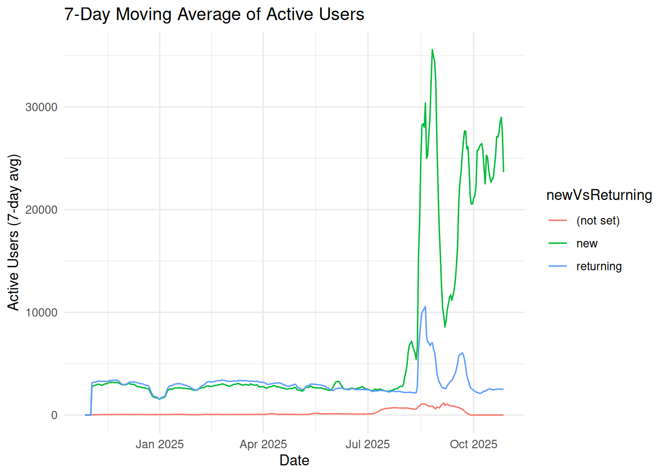
# Plot the moving average for active users
moving_avg_data |>
group_by(date, newVsReturning) |>
summarise(activeUsers_7day_avg = sum(activeUsers_7day_avg, na.rm = TRUE)) |>
ggplot(aes(x = date, y = activeUsers_7day_avg, color = newVsReturning)) +
geom_line() +
labs(
title = "7-Day Moving Average of Active Users",
x = "Date",
y = "Active Users (7-day avg)"
) +
theme_minimal()
#> `summarise()` has grouped output by 'date'. You can override using the
#> `.groups` argument.